3D-printed Microscope Build

1 Learning Objectives

By the end of this lab you will have…

Built your own microscope
Learned how to control the LED array from the Raspberry Pi
Captured an image and analyzed it to determine the resolution of the optical system.

2 Setup

In this section you will put together the individual components for your microscope that are in your kit. This consists of printing the mount, soldering the LED array and Raspberry Pi headers, and assembling the parts with the screws and springs included in your kit.

The microscope you will build is based on the microscope developed by Tomas Aidukas, Regina Eckert, Andrew R. Harvey, Laura Waller, and Pavan C. Konda in their 2019 paper “Low-cost, sub-micron resolution, wide-field computational microscopy using opensource hardware“. You can read the paper here and access the supplementary information here.

Figure 1: A photo of the finished 3D-printed microscope.

2.1 Makerspace 3D Printer Room Access

Before printing the parts for your microscope, you’ll need to get access to the 3D printing room in the Makerspace if you haven’t done so already. You will need to read two policies and take the associated quizzes: the General Use Policy and the 3D printer policy. After finishing the quizzes, you should shortly receive swipe access to the 3d printer room.

2.2 Printing the Microscope Body

To build your microscope you’ll need to print out the individual parts on the 3d printer. You can use the Original Prusa i3 MK3S+ PLA printers in the HMC Makerspace. To print them, you’ll need the stereolithography (.stl) files. The files are available in the shared folder here under the stl subdirectory. The scad files used to generate the stl files are also included in the folder in the scad subdirectory. If you wish to make any modifications or experiment with the files, you can download OpenSCAD and view the files.

After downloading the files, you’ll need to prepare the prints on the printers in the Makerspace. Either the “0.3 mm DRAFT” or “0.15 mm SPEED” print settings should print at sufficient resolution and a reasonable amount of time.

To print the files, you will use the PrusaSlicer software. This software takes the .stl files and slices them into layers which are then translated into directions telling the printer where to move to lay down the individual layers for your object. These instructions for the Prusa printers are written in a file format called .gcode files, which are commonly used in applications for Computer Numerical Control (CNC) machines that are needed by the printers. After slicing and creating the .gcode files, they must be transferred to an SD card and inserted into the SD card slot on the printers in order to print the files.

The easiest way to print is to use the computer in the Makerspace 3D print room directly to slice and export the files for the printers since the profiles are already configured properly. You can download a copy of the .gcode file for all the required parts here. If you open this in PrusaSlicer you will see all the parts arranged on the build plate. I’ve printed this on the printer with success, but it’s a little risky because you are doing everything in one shot so if the print fails, you may have multiple failed parts.

If you wish, you may also print the parts individually by manually adding them to the build plate using the menu option “File > Import > Import STL/OBJ/AMF/3MF…” option. This will allow you to individually add the parts.

Figure 2: A screenshot of the Import menu in PrusaSlicer.

Then you’ll need to move and rotate them to place them on the build plate. Note that you’ll want to orient the parts so that you minimize the number of overhangs since the 3D printer build layer upon layer from bottom to top. Sometimes these are unavoidable though (like on the structure.stl part) and this is ok most of the time even though the print quality for those overhangs is a bit less polished.

You can log on to the computer on the left side of the desk to the right of the printers along the wall. Then either download the files from the web to the computer or transfer them using a USB thumb drive. Open them in PrusaSlicer and add them to the build plate. You can print all of the parts together in a single print using the

2.3 Assembling the Microscope

After all the parts have been printed, you need to assemble the microscope. There are two main sub-assemblies: the bottom structure which holds the LED array and Pi and the top assembly which holds the spring-loaded camera and lens holder which slides up and down to focus.

See the instructions here starting on line 115 describing how to assemble parts.

2.3.1 Installing the Camera Assembly

The camera module is fragile and sensitive to static discharge, so try to touch a large grounded metal object (e.g., metal table, faucet, etc.) before beginning this section.

To achieve a ~1.5x magnification with the lens currently on the camera you need to remove the camera lens and displace it from the sensor by a few mm. To remove the lens, carefully use the circular white plastic tool that came with the camera to unscrew the lens. Then take the lens all the way off. If your camera module is not already secured to the PCB, remove the small plastic sheet covering the adhesive tape on the back of the module and firmly press it onto the PCB.

After removing the lens, press it into the camera mount with the small aperture facing toward the bottom (in other words, oriented in the same way with respect to the camera sensor as it originally was, just now at a larger offset). Then, attach the camera PCB to the camera mount using the small M1.4 screws in your kit. Make sure the camera cable port is facing out from the trapezoidal side of the mount which connects to the holder.

2.3.2 Installing the Camera Mount

Next slot the camera mount into the mount holder. You may need to slightly stretch the springs if you are having trouble getting them mounted. It is easiest to first connect them to the base of the camera mount using the bar on the bottom and then pushing the entire camera mount unit up in order to get the top side of the springs to attach to the holder near the focus adjustment screw.

After you finish this step, the entire camera mount is finished. Attach it to the flat top piece using two M6 screws. You may need bolts as well, but normally screwing it into the plastic holes is sufficient.

2.4 Soldering the DotStar LED Array

The LED array you have in your kit is the 8x8 DotStar Array from Adafruit. This is a very bright array of RGB LEDs. The array comes with a capacitor which can be used as a decoupling capacitor to smooth out any fluctuations in the power supply voltage. You also have a 4-pin, right-angle male header strip. Before soldering the headers on, use two pairs of needle-nose pliers to bend the header into an S shape. Then solder the short half of the header onto the circular pads on the bottom of the LED array PCB. You will connect to these headers with your hookup wire to connect the LED array to your Raspberry Pi.

Figure 3: A photo of the bent right-angle header.

2.5 Soldering the Pi Header

Your Raspberry Pi comes with a spot on the board to connect a 2x20 header. You have a 2x20 right-angle female header which you will need to solder to this connection.

2.6 Connecting the LED Matrix

After soldering it, you can connect the Raspberry Pi to your LED matrix using the jumper wires in your kit. Before making any connections, disconnect your Pi from USB power.

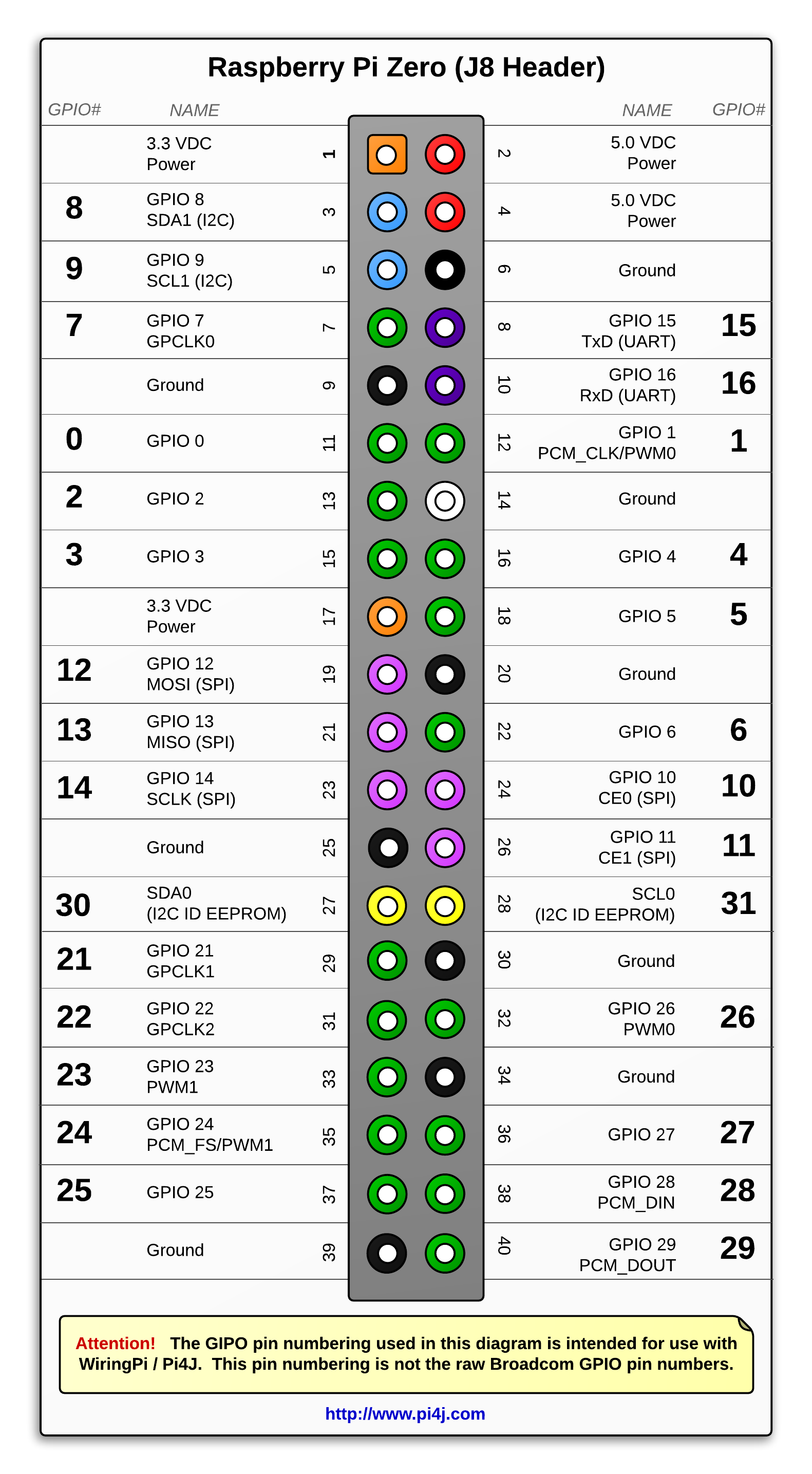
See the instructions here for the pinout, connection diagram, and instructions on using the library. The DotStar array is controlled using the hardware SPI interface on the Pi. Power the LED array by connecting the 5 V and GND pins to the 5 V and GND pins on your Pi. Then connect the SDI pin on the array to the MOSI pin on the Pi (pin 19) and the SCL pin to the array to the SCLK pin on the Pi (pin 23). See the diagram here as a reference. Make sure to double check your connections (best to have a friend check!) to make sure you have everything connected properly before powering it up.

In addition to connecting the array to the correct pins, you’ll need to enable the SPI interface in the Pi configuration menu. Run sudo raspi-config and enable SPI under the “Interface Options” sub-menu.

2.7 Mounting the LED Array

Because the LED array is 8x8, there is no natural center LED. To fix this, the LED array mount is shifted by half an LED pitch up and to the right. This means that the array is now centered at pixel index (3,3) which is the pixel in the 4th row and 4th column counting from the bottom left since the indexing starts at 0. Pixel (0,0) should be located in the bottom left corner when viewing the microscope from the side away from the translation stage. See photo below where LED (0,0) is illuminated. So, to use only a 7x7 subset of the matrix, we should only write to the first 7 rows and columns row_idx = [0,6] and col_idx = [0,6].

Figure 4: A photo showing the correct alignment of the LED array.

3 Blinky Blinky

After setting up your microscope, the first thing we will do is test out the LED array. Activate the virtual environment you set up in Lab 1 (by running source ./.env/bin/activate in your shared directory). Then, we need to install the libraries for the DotStar array (documentation found here). To install it, run sudo pip3 install adafruit-circuitpython-dotstar in your virtual environment. After installing, open up a Python prompt and run the following lines of code.

import board
import adafruit_dotstar as dotstar
N_dots = 8*8
dots = dotstar.DotStar(board.SCK, board.MOSI, N_dots, brightness=0.05)

After importing libraries and creating the DotStar object, try lighting up some single LEDs using a line following the syntax below.

led_idx = 10
dots[led_idx] = (255, 0, 0)

See if you can figure out the indexing of your array to turn on the LEDs near the center of the array. You can turn off the LED either by writing it to zero (0,0,0) or using the built in functions to clear the array.

Create scripts in Python to do each of the following. In this lab we’ll only use the red channel, so you only need to support turning on the red LEDs in the matrix. - Turn on all the LEDs at the same time - Turn on a single LED at a specified x,y location

4 Microscope Image Capture

After figuring out how to control your LED array, the next thing we will do is to take an image and analyze it. For all of these images we will do our analysis using red illumination and only take the data from the red channel of the raw Bayer data.

4.1 Resolution Calculation

To measure the resolution of our microscope we will us a standard optical target called a US Air Force (USAF) target. You may read more about the targets here. This target has sets of bars at decreasingly small pitches or separations. These can be used to determine the finest feature size that can be resolved by the optical system. We will talk much more about resolution in future weeks, but for now, you just need to know that the resolution of an optical system is determined by two quantities: the wavelength and the numerical aperture (or equivalently angular acceptance range) of the optical system.

To determine the overall resolution of the system we need to take an image and then look at the set of bars with the smallest resolution that we are able to resolve. There are several technical criteria to specific the resolution (e.g., Abbé, Sparrow, Rayleigh), each with their own respective equations, but for the context of this lab we will use Abbé’s definition.

\[ d=\frac{\lambda}{(2 n \sin⁡(\theta)}=\frac{\lambda}{NA_\text{illumination} + NA_\text{collection}} \]

Solving this equation for \(d\) yields the minimum distance that can be resolved by our optical system.

For our optical system, using the definitions above, answer the following questions:

What is the NA of the microscope (recall from Lab 2 or calculate the NA from the f-number and aperture diameter)?
What is the maximum value of the NA in air?
What is the minimum resolvable distance \(d\) using red illumination (~630 nm) and the maximum NA in air calculated above?
What is the minimum resolvable distance \(d\) using red illumination (~630 nm) and this microscope?

4.2 Resolution Analysis

In this section you will take an image of the USAF target using your microscope and analyze it. Set up your microscope and turn on all the red LEDs. Then, using VNC, use the command line preview tool libcamera to preview the camera by running “libcamera-still -t 0”. This takes an image with an infinite timeout. To exit the window, use ctrl + c. Adjust the focal screw to bring the image into the sharpest focus you can and then exit the preview.

Figure 5: R1DS1P - Positive 1951 USAF Test Target, Ø1” from Thorlabs (link)

Take a raw Bayer image of the sample and save it to a .npy file. To capture consistent images, make sure to

Turn off the automatic exposure setting by setting the exposure_mode property of the PiCamera object to “off”
Set the shutter_speed property to a value which maximizes the dynamic range of the image you capture. In other words, choose a value for the exposure time such that the maximum value of your image spans nearly the whole range of values available for each pixel (you can calculate this value using the bit depth. For example, for an 8-bit depth your pixels can range from 0 to \(2^8-1=255\). You should shoot to have the max value of your image reach to roughly 90% of the maximum value without exceeding the value and clipping).

After taking the image, transfer the file to your host machine, load it into Python, and plot the red channel. You’ll notice that the raw red channel is sparse (i.e., 75% of the pixels are black). This is because of the Bayer array which splits the channels into red, green, and blue pixels.

Before performing your analysis, write Python code to process the raw Bayer data from the red channel and remove the zero entries as shown in the figure below.

Figure 6: Bayer color filter array single channel selection

Using the processed image of the red channel, answer the questions below:

What is the effective pixel pitch of the red channel images on the camera sensor plane (i.e., what is the distance between adjacent red pixels?)?
What is the effective pixel pitch of the red channel images on the object plane?
What is the sampling frequency of your image sensor at the sample plane in cycles per millimeter (i.e., the inverse of the pixel pitch at the object plane).
Given the minimum detectable feature size \(d\) for this microscope from the Abbé resolution equation earlier, what spatial frequency does this correspond to?
Does your camera sensor satisfy the Shannon-Nyquist sampling theorem requirement that the sampling frequency must be twice the maximum spatial frequency in the sample field?
What is the minimum resolvable feature in the image? To determine this, create a zoomed-in image of a region of interest of the USAF target where you can start to see the bars blur together. The size of the smallest bar separation that you can measure is a good estimate of your system resolution.
Save a copy of your zoomed-in ROI image. Make sure to follow good presentation practices and include a scale bar, a figure title, axis labels, and a colorbar.
Create a 1D plot of the intensity of perpendicular to three bar target: one that is clearly resolved, one that is just barely resolved, and one that is unresolved. See Figure 3 from the paper for an example of the types of plots that we are looking for here.